Question 1 (d)
Degrees of price elasticity of supply
9 marks
- Time to write
- About 18 minutes
Question
Question 1 (d) · 9 marks"Elasticity of supply measures how responsive the supply of any goods is to change its own price". With this statement in view, explain with a diagram the different degrees of price elasticity of supply.
Reworded from the university paper; the task is the same. The original paper belongs to the University of Delhi. See DU's question bank.
Before you write
Read off the question and its marks
Read from the question
- statementTie the answer to the quoted statement: say what it means first, and come back to it at the end.
- diagramDraw the diagram, and label both axes and every curve.
What the paper leaves open
"To change its own price" stands as printed; it is read as "to a change in its own price".
Write it in this order
- Read; underline the asks; jot your points 1 min
- 1 Meaning and formula 2 marks 4 min
- 2 Five degrees, each with its diagram 5 marks 9 min
- 3 Factors deciding the degree, and conclusion 2 marks 3 min
- Check: every ask answered, key terms underlined 1 min
Easy marks
- Step 1 opens with the meaning: a one-line definition, the quickest mark in it.
Short on time? Trim steps 1–3 evenly rather than skip one: each is capped at its own marks.
Try it first. About 18 minutes for 9 marks. Write it out, then open the solution.
Solution
Hover or tap a marked figure, like 72,000, to see how it is made and where else it appears.
Price elasticity of supply measures how strongly the quantity supplied of a good responds to a change in the good's own price, other things remaining the same:
Eₛ = (percentage change in quantity supplied) ÷ (percentage change in price) = (ΔQ/Q) ÷ (ΔP/P).
Because the supply curve normally slopes upward, Eₛ is positive. Its size tells us how far producers can and will adjust output when the price moves. On a straight-line supply curve there is a simple test: a line that, extended, starts from the price axis is elastic, one that starts from the origin is unitary, and one that starts from the quantity axis is inelastic.
Degrees of price elasticity of supply
In each diagram price is on the vertical axis and quantity supplied on the horizontal axis. The five degrees are easiest to see by starting from the dividing line, Eₛ = 1, then taking the two cases found in most markets on either side of it, and ending with the two extreme, limiting cases.
The dividing line
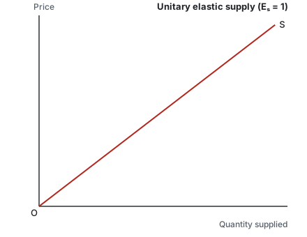
- Unitary elastic supply (Eₛ = 1), Figure 3. Output and price move by equal percentages: a 10% rise in price brings exactly a 10% rise in quantity. Every straight-line supply curve drawn through the origin behaves this way, which makes it the benchmark against which the other cases are judged.
The two ordinary cases
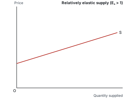
- Relatively elastic supply (Eₛ > 1), Figure 4. Producers respond strongly: the percentage rise in output is bigger than the percentage rise in price. The curve is fairly flat, and if extended it cuts the price axis. Example: ready-made garments or plastic buckets, where spare machines and labour let output be stepped up fast.
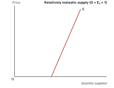
- Relatively inelastic supply (0 < Eₛ < 1), Figure 2. Producers respond only weakly: output grows by a smaller percentage than price. The curve is steep, and if extended it cuts the quantity axis. Example (our own): hotel rooms in a hill town in the summer season; a higher tariff fills the rooms that already exist, but no new rooms can come up before the season ends.
The two limiting cases
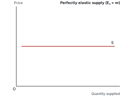
- Perfectly elastic supply (Eₛ = ∞), Figure 5. The curve is flat, a horizontal line at one price. At that price sellers offer whatever quantity is wanted; let the price slip even a little below it and they offer nothing. A competitive industry working under constant costs in the long run fits this case.
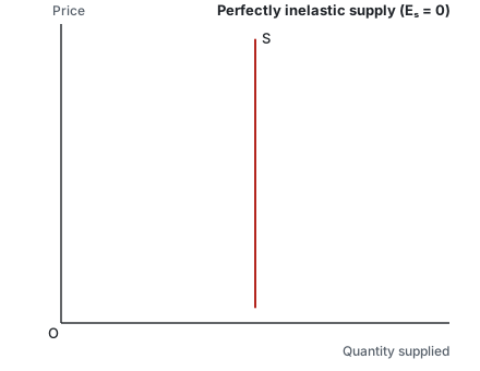
- Perfectly inelastic supply (Eₛ = 0), Figure 1. The curve stands upright, a vertical line at a fixed quantity: however far price moves, not one more unit is offered. Example: the seats in a stadium for one match, or a perishable catch of fish already landed for the day.
- Time: supply is more elastic the longer producers have to adjust (very short period, short run, long run).
- Spare capacity and stocks: idle machines or unsold stocks let output rise quickly.
- Mobility of inputs: inputs that move easily between uses make supply more elastic.
- Nature of the good: perishable goods have inelastic supply in the very short period; easily stored or easily produced goods have elastic supply.
- Behaviour of costs: if costs rise sharply as output expands, supply is inelastic.
Price elasticity of supply runs from zero (vertical curve) through one (a line through the origin) to infinity (horizontal curve). For a business it shows how far output can follow a price rise: a producer with elastic supply can take advantage of higher prices, while one with inelastic supply mostly sees the price rise as higher revenue per unit.
Where the 9 marks sit
| # | Component | Marks |
|---|---|---|
| 1 | Meaning and formula | 2 |
| 2 | Five degrees, each with its diagram | 5 |
| 3 | Factors deciding the degree, and conclusion | 2 |
| Total | 9 |
Report a problemopens an email to admin@getkunji.com with the question ID7506-Q1dalready filled in.